 Weld Fatigue
Table of contents
About Fatigue
The weld fatigue methods are based on IIW recommendations to evaluate fatigue according to Nominal, Hot-Spot, Effective Notch methods. The new code EN 1993-1-14:2025 Eurocode 3 chapter “8.2 Fatigue” can also be used to learn more about the three methods above.
Three additional generic fatigue methods CSV stress, Linearized stress and Structural stress fatigue method are included that can be used for user defined evaluation of e.g. structural stress fatigue of welds according to DNV or pressure vessel evaluation according to ASME. The list of fatigue methods and supported geometry and location (Node/Element) is shown below.
| Fatigue Method | Shell | Solid | Node/Element |
|---|---|---|---|
| CSV Stress | Yes | Yes | Yes/Yes |
| Linearized Stress | No | Yes | Yes/No |
| Structural Stress | Yes | Yes | Yes/Yes |
| Nominal Stress | Yes | Yes | Yes/No |
| Hot-Spot Stress | Yes | Yes | Yes/No |
| Effective Notch Stress | No | Yes | Yes/No |
Load cases from single step, load case combination/scanning or solution combination/scanning can be defined.
Mean stress correction according to Goodman, Soderberg, Gerber, ASME Elliptical and Modified Goodman can be used in CSV, Linearized, Nominal and Hot-Spot method.
Cumulative Damage from a duty cycle consisting of several load cases can be evaluated.
S-N curves from IIW, DNV GL RP-C203, and Eurocode 3/9 are included, and additional curves can be added. Fatigue evaluation using a S-N curve works in the same way as Ansys fatigue tool, but the difference is that the Ansys tool is used for the part material fatigue excluding welds.
Common fatigue properties
The common properties for all fatigue methods, (S-N curve, Load case definition, Fatigue Result and Definition) are described in the following sections.
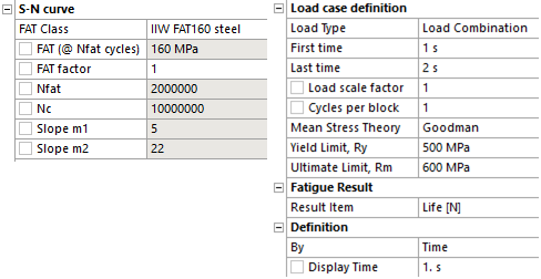
| S-N curve | |
|---|---|
| FAT Class | Select a FAT class (i) |
| FAT factor | Scale factor for FAT value (Default 1.0). E.g. to apply a thickness or temperature modification factor. (ii) |
| FAT (@ Nfat cycles) (*) | Stress range at Nfat cycles |
| Nfat (*) | Number of cycles for defining FAT |
| Nc (*) | Number of cycles break point between slope m1 and m2 |
| Slope m1 (*) | S-N curve slope m1 for N < Nc |
| Slope m2 (*) | S-N curve slope m2 for N > Nc |
| S-N Table (i) | Tabular editor for S-N data |
| Ncutoff | Maximum calculated life |
| Load case definition | |
| Load Type | Select a Load Type (Default “Fully Reversed”) |
| Loading Ratio | Factor to define custom range. Visible for Load Type “Ratio”. (Default = -1 Fully Reversed) |
| First Time | Visible for all Load Type but “Solution Combination”, “Solution Scanning” or “Random”. (Default = 1.0) |
| Last Time | Visible for Load Type “Load Combination” and “Load Scanning”. (Default = 0.0) |
| Solution Editor | Table editor. Visible for Load Type “Solution Combination” and “Solution Scanning”. |
| Load scale factor | Fatigue stress scale factor. Visible for all Load Type except “Random”. (Default = 1.0) (ii) |
| Cycles per block | Number of cycles used to calculate damage and safety factors. Visible for all Load Type except “Random”. (Default = 1) |
| Exposure Duration | Duration of the Random Vibration load (in seconds). Visible for Load Type “Random”. (Default = 3600 sec) |
| Statistical Average Frequency | The Random Vibration Statistical Average Frequency, SAF. Visible for Load Type “Random”. Used to calculate the number of cycles based on the Exposure time (iii). |
| Mean Stress Theory | None (default)/Goodman/Soderberg/Gerber/ASME Elliptical/Modified Goodman/Eurocode 3 |
| Yield Limit, Ry | Material Ry, Used for static stress check for _Nominal and Hot-Spot method. |
| Ultimate Limit, Rm | Material Rm, Visible for Goodman/Gerber/Modified Goodman |
| Fatigue Result | |
| Result Item | Weld Result Item |
| Display Graph | No (Default)/Yes. If Geometry are edges the path result is displayed in the Graph window. |
| Definition | |
| By | Time (Cannot be changed) |
| Display Time | Time step selected from “First Time” in Load case definition (Read only). |
(i) FAT Class
The default FAT Class for each fatigue method is defined in the Weld Fatigue Settings.
The list of FAT Classes can be edited in Weld Settings using FAT Class Editor.
Use “User defined” to edit S-N curve properties manually (otherwise the properties marked with (*) are in read only mode).
Use “User defined S-N Table” to create a manual S-N Curve using the S-N Table.
Tip: Start typing to filter the list!
(ii) FAT factor & Load scale factor
EN 1993-1-9:2025 Eurocode 3 uses “partial factors” to scale applied stress range and fatigue resistance.
Partial factor for applied stress ranges: γFf = Load scale factor
Partial factor for fatigue resistance: γMf = 1/FAT factor
(iii) Statistical Average Frequency
The Statistical Average Frequency, SAF, is defined as the ratio of the RMS Stress Velocity Result and the RMS Stress Result; SAF = (σrms v/σrms u)/(2π). It is also possible to use the ratio of RMS Velocity and RMS Displacement in the dominating response direction that contributes to the stress.
For “CSV”, “Structural” and “Linearized” method the value of SAF must be defined.
For “Nominal”, “Hot-Spot” and “Effective Notch” methods the value of SAF is calculated automatically and the value is stored as Result Item “Last time”.
S-N Curve
The FAT Class S-N curve data can be of two types, bi- (or tri-) linear using a FAT value and slope parameters m1 and m2 or a generic S-N Table of data. When selecting a FAT Class defined as a S-N Table the values are loaded and can be viewed/edited clicking the “Tabular Data”.
The default FAT Class properties for Nominal, Hot-Spot and Notch method are shown in the figure below. Use the FAT Class Editor in Weld Settings to add or edit the FAT classes.

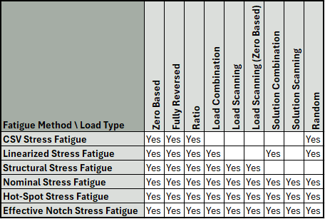
Load Types
The available Load Types for each Fatigue Method is shown in the figure below.
-
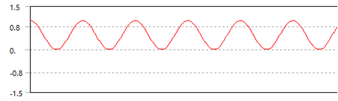
Zero Based
Calculates a pulsating stress range by scaling load step First time with Load scale factor.
-
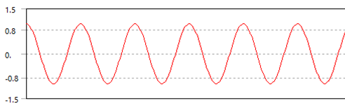
Fully Reversed
Calculates an alternating stress range by scaling load step First time with 2*Load scale factor.
-
Ratio (Loading Ratio) (i)
Calculates custom stress range defined by scaling load step First time with (1 - Ratio)*Load scale factor.
-
Load Combination
Calculates the stress range between step First time and Last time and scale with Load scale factor.
-
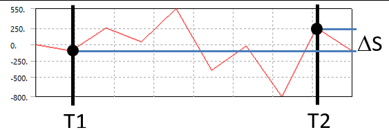
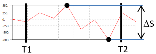
Load Scanning(ii)
Calculates the maximum stress range between step First time and Last time and scale with Load scale factor.
-
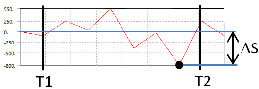
Load Scanning (Zero Based)
Calculates the maximum stress range from each individual load step between step First time and Last time and scale with Load scale factor.
- Solution Combination
A general load step combination with two or more load steps from any analysis in the model tree. The sum of the steps defines the stress range.- To edit the Solution Editor click on “Tabular Data”
- Click the “Add row” in the table editor
- Select analysis name. (Default “Current Analysis”)
- Define the time step (must be greater than 0)
- Define the load step scaling coefficient (must not be 0)
- To delete a row right-click on a cell and select “Delete selected row(s)”
- Click “Apply” to save the data and close the table editor.
- (Click “Cancel” to close without saving). Do not click the red “Close window” button.
The sum can be scaled with Load scale factor

-
Solution Scanning (ii)
Calculates the maximum stress range within all possible combinations of the selected steps in the Solution Editor. - Random (iii)
Calculates the damage in a Random Vibration (Spectrum) analysis using the Steinberg Formulation.
This method is only valid in a Random Vibration analysis except for the CSV Method that also can use it in Static and Transient analyses.
(i) Loading Ratio vs. Stress Ratio
The Load Type “Loading Ratio” defines the scaling factors, Kmin & Kmax, from the Ratio for the selected load case, LC, according to the following:
Ratio = Kmin/Kmax , where Kmax = 1.
Range = Kfact·(Kmax·LC – Kmin·LC) = Kfact·(1-Ratio)·LC, where Kfact is the Load scaling factor.If the stress in a point for the selected load case is negative, e.g. S = -100, and Ratio = -0.5 the stress range is,
Srange = abs(1·-100 – -0.5·-100) = abs(-100 – 50) = 150
The stress ratio, R = Smin/Smax = -100/50 = -2!
If the stress in a point is positive, e.g. S = 100, and Ratio = -0.5, then:
Srange = abs(1·100 – -0.5·100) = abs(100 + 50) = 150, R = 50/100 = 0.5!The “Loading Ratio” will equal the “Stress Ratio” only in points where the stress is positive! Defining a load as a “Zero based” or “pulsating” load may in some points create stresses with R = 0 and in other points R = -inf depending on the stress sign in the load case!
The “Loading Ratio” definition follows Ansys Fatigue Module definition.
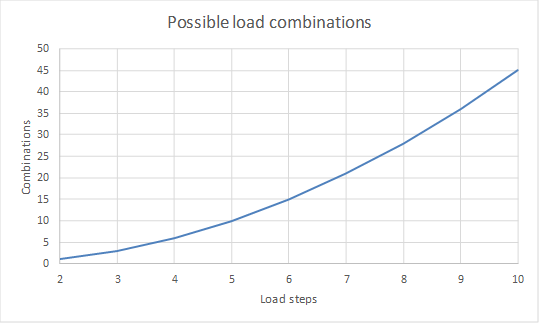
(ii) Load/Solution Scanning evaluation time
Load/Solution scanning performs all possible load case combinations from the selected range of time steps (or load cases in the Solution Editor) in order to find the true maximum principal or equivalent stress range.
The number of combinations increase fast with number of load steps, which is why this feature should be used with care to avoid long evaluation times.
When using a Normal stress type in Nominal, Hot-Spot or Effective Notch stress method the stress orientation is constant for all steps, so the min and max stress are found direct from “Maximum/Minimum over time” and the stress range is derived without performing load case combinations.
(iii) Random
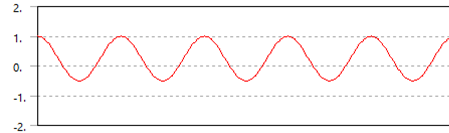
The Steinberg Formulation utilizes all three stress occurrences (1σ, 2σ, 3σ) and their rate of occurrence along with the Miner’s rule in order to compute the total fatigue damage, D, of the system based on the Exposure Time, t, and Statistical Average Frequency, SAF.
D = n1σ/N1σ + n2σ/N2σ + n3σ/N3σ
Where:
n1σ = 0.6827·SAF·t; actual number of cycles at or below the 1σ level (68.27%).
n1σ = 0.2718·SAF·t; actual number of cycles at or below the 2σ level (95.45% - 68.27%).
n1σ = 0.0428·SAF·t; actual number of cycles at or below the 3σ level (99.73% - 95.45%).
and N1σ, N2σ and N3σ are the corresponding number of cycles at the stress levels 1σ, 2σ, 3σ.
Mean Stress Correction Theory
Mean stress correction, MSC, can be applied if the Load type is one of Zero-based, Ratio, Load Combination, Load Scanning, Solution Scanning. If Load type is one of Fully Reversed, Solution Combination or Random the mean stress is by definition zero and the selected MSC will have no impact on the results.
The definition is the same as in Ansys Fatigue Module except for “Modified Goodman” and “Eurocode 3” (that is not available in Ansys Fatigue Module). If the mean stress is outside of the Yield or Ultimate limit a warning message is issued and the stress range is assigned a large value and the life is set to 0 cycles.
Based on the mean stress, Savg, the stress range, Srange, is corrected according to the following equations:
- Goodman: S’range = Srange/(1 - Savg/Rm) if 0 < Savg < Rm
- Soderberg: S’range = Srange/(1 - Savg/Ry) if 0 < Savg < Ry
- Gerber: S’range = Srange/(1 - (Savg/Rm)2) if abs(Savg) < Rm
- ASME Elliptical: S’range = Srange/sqrt(1 - (Savg/Ry)2) if 0 < Savg < Ry
- Modified Goodman: S’range0 = Srange/(1 - Savg/Rm) if -Rm < Savg < Ry
if Savg > 0: S’range1 = S’range0·(0.5·Srange/(Ry - Savg))
elif Savg <= 0: S’range1 = S’range0·(0.5·Srange/(Rm + Savg))
S’range = max(S’range0, S’range1) - Eurocode 3:
if Savg < -0.5·Srange: S’range = 0.6·Srange
elif Savg < 0.5·Srange: S’range = 0.4·Savg + 0.8·Srange
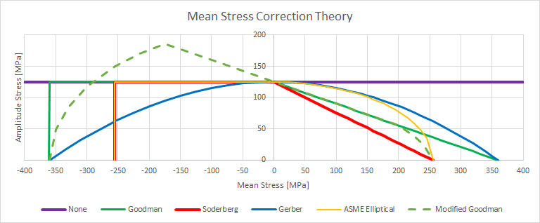
The Modified Goodman uses a two step approach to first derive a corrected range using Goodman equation and then modify the range based on average stress distance to Ry or Rm.
The Eurocode 3 follows “7.4 Effective design value of stress range” EN 1993-1-9:2025 Eurocode 3 but is re written to use Savg and Srange instead of Smin and Smax.
The Load types “Fully reversed”, “Solution Combination” and “Random” has by definition zero mean stress and is not influenced by the mean stress correction.
Fatigue Result
The result items are listed in the table below and are also marked in the “S-N curve” figure above.
When selecting the “Life [N]”, “log10(Life) [N]” or “Safety factor stress” the legend is set to “Reversed Rainbow” and optionally “Logarithmic” and “High Fidelity”. The automatic legend does not modify the legend in the related Figure, but it can be disabled in the Weld Settings “Automatic Weld Fatigue Legend = No”.
| Result Item | Description |
|---|---|
| Life [N] | Number of cycles for failure at defined stress range, N(Δσ). |
| log10(Life) [N] | Convenient method to plot the order of magnitude of life, log10(N(Δσ)). |
| Damage per block [-] | Ratio of Cycles per block to calculated Life, D = Nb/N(Δσ). |
| Safety factor life [#blocks] | Number of loading blocks, SFN = 1/D = N(Δσ)/Nb. |
| Stress range | Stress range, Δσ (i). |
| Safety factor stress | Ratio of allowed stress range to Stress range, SFS = Δσ(Nb)/Δσ. |
| Stress utilization | 1/SFS = Δσ/Δσ(Nb) |
| Life Quality | Quality measure based on mesh size. |
| Stress max | Maximum stress in the fatigue load case. |
| Stress avg | Average (mean) stress in the fatigue load case. |
| Stress min | Minimum stress in the fatigue load case. |
| First time | First of the identified time steps when using “Fatigue Scanning” or “Solution Scanning”. |
| Last time | Last of the identified time steps when using “Fatigue Scanning” or “Solution Scanning”. |
| Path pos | Path coordinate along geometry edge. (ii) |
(i) Stress range
For “Zero based”, “Fully Reversed” and “Ratio” load cases the sign of the stress range can be kept to indicate if loading is in tension (positive) or compression (negative). To enable this set Weld Fatigue Settings option “Signed stress range = Yes”.
(ii) Path pos
Each fatigue result can display the selected result item in the Graph window using the new property “Display Graph = Yes” if the Geometry scoping is “Edge”.
Display Graph
For a fatigue result with one continuous set of edges a path plot of the selected Result Item can be displayed in the Graph window. The output csv file is sorted with the “Path pos” for each group of edges.
The direction of the path is decided by the first two edges in the Geometry scoping.
 CSV Stress Fatigue
About
The CSV Fatigue Method is a generic post processing method to evaluate the life result items based on nodal or element stress values in a CSV text file (comma separated values).
Usage
The first column in the csv file must contain node or element numbers. At least one column must contain stress results. The first (non-empty) line must contain data headers with valid Workbench unit strings, e.g. [MPa] or (Pa). Both types of brackets may be used around the stress unit. Blank lines and lines beginning with “#” are ignored. The field separator may be “;” or “,”. If the separator “;” is used decimal comma “,” or decimal point “.” may be used. If the separator “,” is used only decimal point “.” can be used.
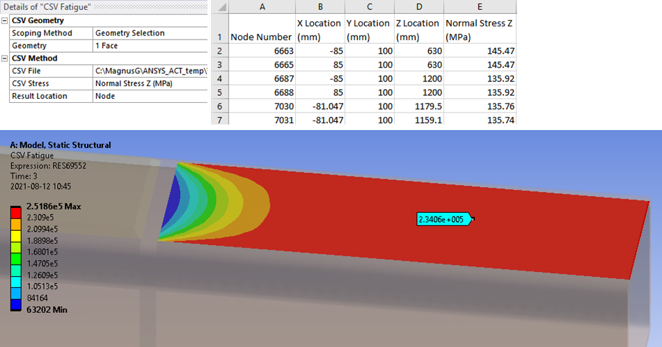
| CSV Geometry | |
|---|---|
| Scoping Method | All Bodies/Geometry Selection/Named Selection |
| Geometry | Selection corresponding to the content in the CSV file (i). |
| CSV Method | |
| CSV File | Open file dialog for external CSV text file. |
| CSV Stress | List box of available stress results. The header must include a valid stress unit string. |
| Result Location | Node (Default)/Element. Set the type according to the CSV file result type. |
(i) Geometry
If the file contains edge results the scoping must be “edges” otherwise the contour plot is blank. You may limit the plot by selecting fewer geometry items.
Load case definition
Only Load Type “Zero Based”, “Fully Reversed”, “Ratio” or “Random” may be used with CSV fatigue.
The selected stress is scaled based on the Load Type and the Load scale factor properties. E.g. If using a CSV Stress that is a “Stress range” you need to apply a scaling factor of 0.5 if using Load Type “Fully Reversed”.
If using the Load Type “Random” the CSV Stress must be the “1 Sigma RMS amplitude” from a “Random Vibration” analysis.
 Linearized Stress Fatigue
About
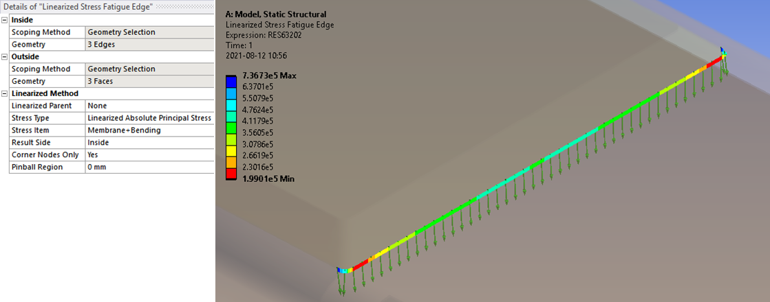
The “Linearized stress fatigue” method is a generic method to evaluate the fatigue based on linearized stress though the thickness of a part, e.g. along a weld toe from inside to outside.
Compared to the native linearized stress feature in Mechanical that uses a predefined path in “Construction geometry” the app defines the needed paths and linearization in the background using MAPDL.
Usage
| Inside (Source) | |
|---|---|
| Scoping Method | Geometry Selection/Named Selection |
| Geometry | Edges, Faces or Nodes of solids on the “Inside”. Results are plotted on this geometry (i). |
| Outside (Target) | |
| Scoping Method | Geometry Selection/Named Selection |
| Geometry | Edges, Faces or Nodes on the “Outside”. For each “Inside” node a path is created to the closest “Outside” node and the linearized stress is evaluated. |
| Linearized Method | |
| Linearized Parent | None/*. Select an existing parent result to evaluate a different stress type, item or result (ii). |
| Stress Type | Linearized Stress Type |
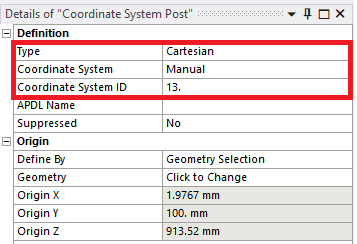
| Coordinate System | [List of Coordinate Systems] Visible for “Normal” & “Shear” Stress (Must be Cartesian with “Manual” ID number and created before solving) (iii). |
| Stress Item | Membrane/Bending/Membrane+Bending (Default)/Peak/Total |
| Result Side | Inside (Default)/Center/Outside]. Result location to display. |
| Corner Nodes Only | Yes (Default)/No. Use to speed up evaluation. |
| Pinball Region | Search distance limit when creating a path between Inside and Outside geometry (iv). |
| Fatigue Result | |
| Create Path | “Click here to create path!” |
| Linearized Stress Result | |
| “Stress Item” (Inside) | “Inside” value from plot at location “Max” |
| “Stress Item” (Center) | “Center” value from plot at location “Max” |
| “Stress Item” (Outside) | “Outside” value from plot at location “Max” |
(i) Inside
By using a subset of the face nodes the evaluation time is greatly reduced. Avoid large face selections.
(ii) Linearized Parent
You may use “Linearized Parent” to quickly display a different Stress Item or Results Item or use a different S-N curve or FAT-factor. No evaluation time needed since the linearized stress files are re-used. A Fatigue Child result may be used to display a different Result Item.
(iii) Coordinate System
(iv) Pinball Region
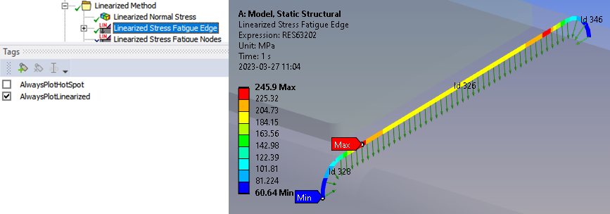
“0” will connect all nodes on the Inside geometry with the nearest node on the Outside geometry. When the result is evaluated, the path is plotted as a green arrow. The arrows can be shown/hidden for a selected result by toggle the tag “AlwaysPlotLinearized”
Linearized Method - Stress Type
| Stress Type | Description |
|---|---|
| Linearized Absolute Principal Stress (Default) | σabs = max(abs(σ1), abs(σ2)), abs(σ3)) |
| Linearized Maximum Principal Stress | σ1 |
| Linearized Middle Principal Stress | σ2 |
| Linearized Minimum Principal Stress | σ3 |
| Linearized Stress Intensity | σint = max(abs(σ1 - σ2), abs(σ2 - σ3), abs(σ3 - σ1)) |
| Linearized Equivalent Stress | σeqv = sqrt(0.5·(σX - σY)2 + (σY - σZ)2 + (σZ - σX)2 + 6·(σXY2 + σYZ2 + σXZ2)) |
| Sum of Linearized Principal Stress | σsum = σ1 + σ2 + σ3 |
| Linearized Normal Stress X | σX |
| Linearized Normal Stress Y | σY |
| Linearized Normal Stress Z | σZ |
| Linearized Shear Stress XY | σXY |
| Linearized Shear Stress YZ | σYZ |
| Linearized Shear Stress XZ | σXZ |
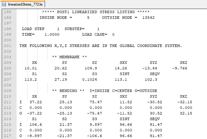
The output from the path evaluation is saved in a text file for each result object in the solution sub folder “Weld Fatigue”.
Fatigue Result - Create Path
Once the result is evaluated a “path object” can be created automatically based on the maximum result using the “Create Path” property. If the result is updated and the max location is changed the path can be updated. This path can be used for additional post processing using the native linearized stress results.
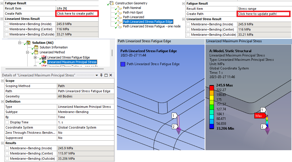
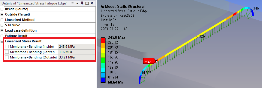
Linearized Stress Result
The stress result details from the linearized stress at the max location are printed as output parameters. The values may differ slightly compared to what Mechanical is displaying and the reason is that the app uses all available nodes and elements in the linearization evaluation in MAPDL whereas Mechanical only uses one body close to the path.
 Structural Stress Fatigue
About
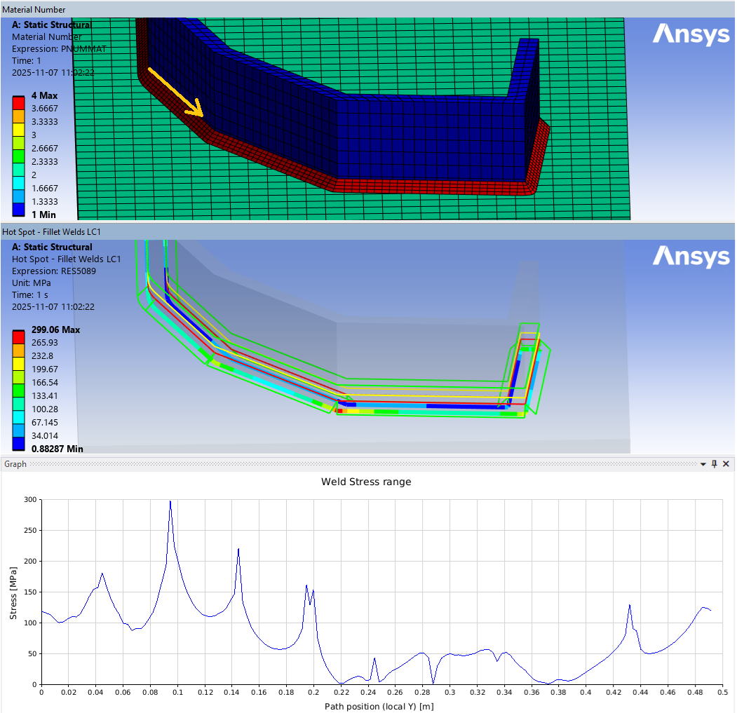
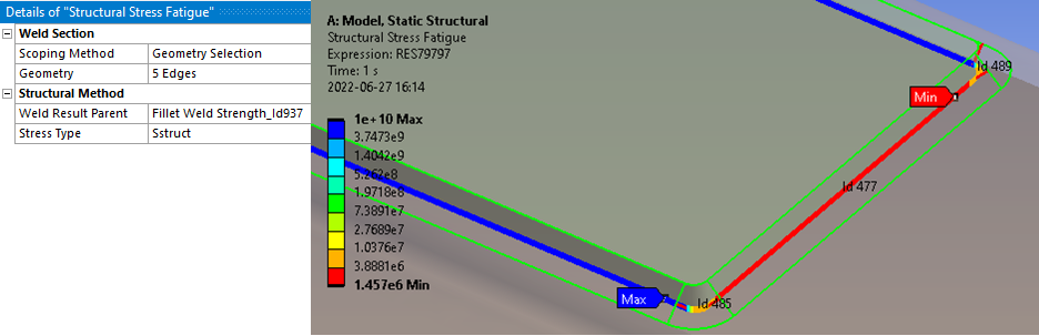
The “Structural stress fatigue” method is used to evaluate fatigue based on the structural stresses in the weld throat defined by a Fillet Weld Strength result.
Usage
| Weld Section | |
|---|---|
| Scoping Method | Geometry Selection/Named Selection |
| Geometry | Edges from selected Fillet Weld Strength result. Results are plotted on this geometry (i). |
| Structural Method | |
| Weld Result Parent | [List of available results] Select an existing Weld Strength Result parent to use for structural stress. (i) |
| Weld Code | Weld Code to use for Seqv calculation. |
| Stress Type | Seqv/Snormal/Sbending/Sstruct (Default)/Sparallel/Stotal/Tparallel/Tnormal/Ttotal See Result Items for description. |
| Result averaging | Local (Default)/Section average stress. |
| Result location | Location of stress (Throat, Leg0, Leg1) Read only property linked to parent result. |
(i) Weld Result Parent
Results based on both Add Fillet/Butt Weld and Geometry Scoping (shell or solid) are valid.
Structural Stress - Stress Type
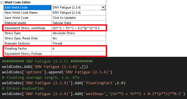
The definition of Stress Type “Seqv” is based on the selected Weld Code and may be different for different codes. The selected Stress Type is also based on the current Result averaging and Floating factor in the selected Weld Result Parent. If using Result averaging = “Section” the “Section (Constant)” weld stress is used in the fatigue evaluation, i.e. one constant value along each weld section edge. It is possible to define a “Weld Strength Code” in the Weld Code Editor (or the “weldStrengthPref.py”) for use with the Structural Stress Fatigue result that only calculates the weld stress “Seqv” and not any weld utilization factor, Wuf. By not defining a “Dimensional Strength” i.e. “FuSeqv” no Wuf is calculated.
S-N curve
It is the user’s responsibility to select a valid FAT Class for the chosen Stress Type. The default Stress Type and FAT Class name may be defined in the Weld Fatigue Settings.
Load case definition
The Weld Result Parent should be evaluated with “Calculate Time History = Yes” so that any load step may be used when defining the “First time” and “Last time” otherwise only the time defined in the parent result is available to use.
If using the Load Type “Random” the Weld Result Parent must be evaluated using “Load scale factor = 1” (1 Sigma RMS amplitude).
 Nominal Stress Fatigue
About
The “Nominal fatigue method” is similar to Ansys Fatigue Tool and can be used to calculate the fatigue on the surface of a part using a selected stress type and S-N curve.
Usage
| Base Material Face | |
|---|---|
| Scoping Method | Geometry Selection/Named Selection |
| Geometry | Edges, Faces or Nodes of shells or solids. (Evaluation is limited to the surface of the part) |
| Shell face | Top(Default)/Middle/Bottom Used only for shell bodies. |
| Nominal Method | |
| Stress Type | Stress Type |
| Coordinate System | [List of Coordinate Systems] Visible for Normal and Shear Stress (Must be Cartesian). The selected stress direction is plotted with a vector. |
| Exclude boundary nodes | Yes (Default)/No. Do not display fatigue results for nodes on boundary conditions. |
Nominal Method - Stress Type
| Stress Type | Description |
|---|---|
| Principal (Default) | σprin = max(abs(σ1), abs(σ3)) |
| Sum of Principal | σsum = σ1 + σ2 + σ3 |
| Stress Intensity | σint = max(abs(σ1 - σ2), abs(σ2 - σ3), abs(σ3 - σ1)) |
| Equivalent | σeqv = sqrt(0.5·(σX - σY)2 + (σY - σZ)2 + (σZ - σX)2 + 6·(σXY2 + σYZ2 + σXZ2)) |
| Shear (Max) | τmax |
| Normal X | σX |
| Normal Y | σY |
| Normal Z | σZ |
| Shear XY | τXY |
| Shear YZ | τYZ |
| Shear XZ | τXZ |
Equivalent is the signed von-Mises Equivalent stress. Sign taken from the largest principal stress.
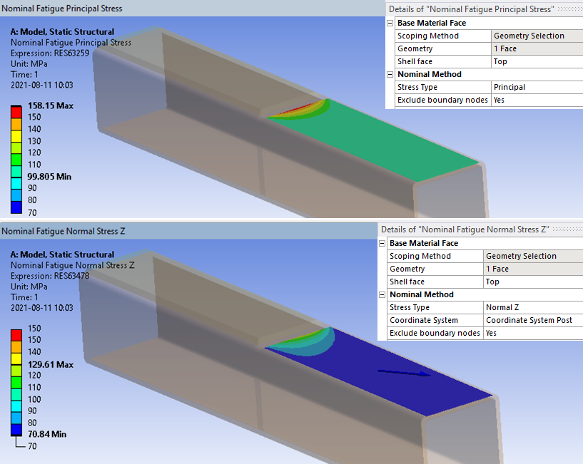
When using Nominal Fatigue for weld fatigue evaluation according to the “Nominal Stress Method” it is the user’s responsibility to read the geometric stress and life at correct location with respect to the selected weld detail, e.g. using the “Normal X” and a local coordinate system.
With the nodal selection (in combination with Normal stress) the user can directly probe the life for a weld joint from a single node without confusing the plot with irrelevant results.
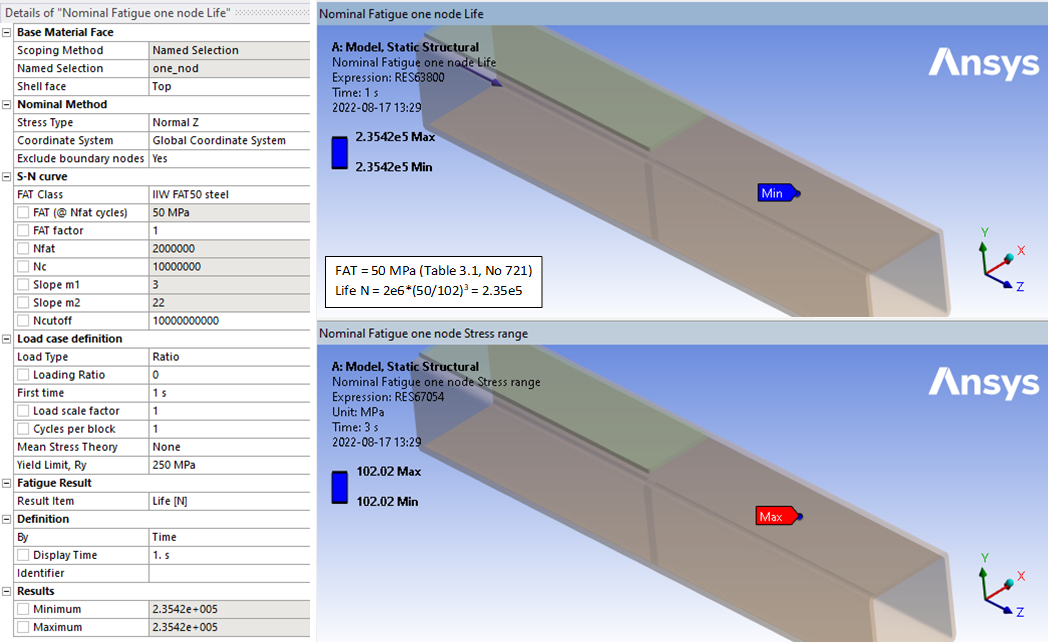
It is important not to read the stress at the weld location (to exclude the influence of the weld itself) and also find correct FAT value. (Structural Details Table 3.1 IIW). It is recommended to use Hot-Spot and/or Effective Notch method for weld evaluation.
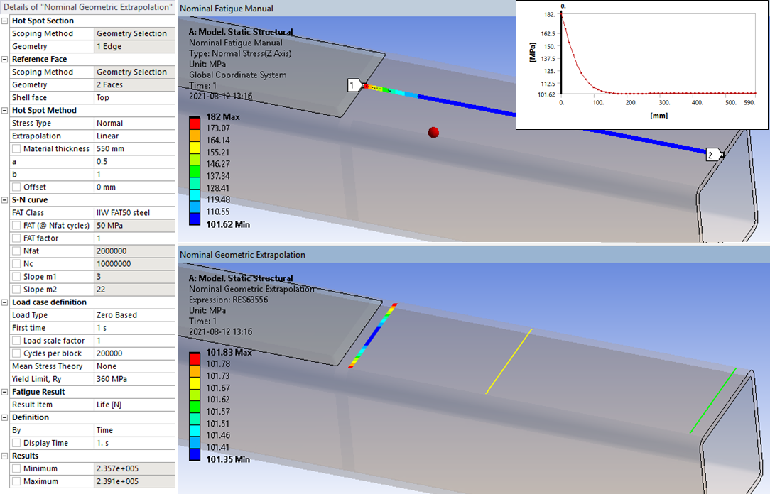
The nominal method does not calculate a nominal stress based on the section forces and cross section area! The Hot-spot method can be used to derive the nominal geometric stress used for nominal fatigue evaluation of welds. The Linearized stress method may also be used to derive the nominal stress in a cross section using the “Result Side = Center”.
The normal stress direction arrow can be shown/hidden for a selected result by toggle the tag “AlwaysPlotNominal”. The default value is defined in the Weld Fatigue Settings.
Geometric Stress Extrapolation
Sometimes it is hard to find the value of the geometrical stress at the weld without the influence of the weld itself. The Hot-spot method may be used to extrapolate the geometrical stress at the weld using two points far from the weld.
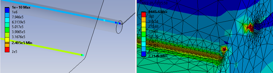
Mesh quality
Nodes from elements connected to a cut boundary section or other displacement constraints are automatically excluded from the evaluation by setting the property “Exclude boundary nodes = Yes”. This sets the “Life quality” to zero and will avoid the stress singularity at the boundary condition to influence the fatigue result, see example below.
The “Life quality” result item is a factor estimating how close to the actual life the calculated life is based on the mesh curvature, see the section Notch Life Quality for more details.
 Hot-Spot Stress Fatigue
About
The Hot-Spot method calculates the maximum stress range at the weld hot-spot (weld toe) by extrapolation of the in-plane surface stress to the hot-spot edge.
Usage
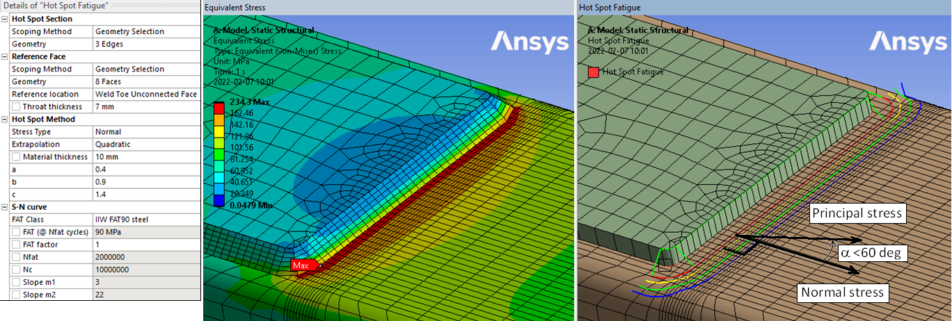
The constant, linear and quadratic method can be used and the extrapolation points, a, b & c, can be edited based on weld code and model thickness, t.
Different weld types and corresponding FAT values are found in Table 3.3 in IIW.
| Hot Spot Section | |
|---|---|
| Scoping Method | Geometry Selection/Named Selection |
| Geometry | Edges along the weld toe, i.e. the “hot-spot”, (Red line). |
| Reference Face | |
| Scoping Method | Geometry Selection/Named Selection |
| Geometry | Reference Faces connected to the hot-spot edges. |
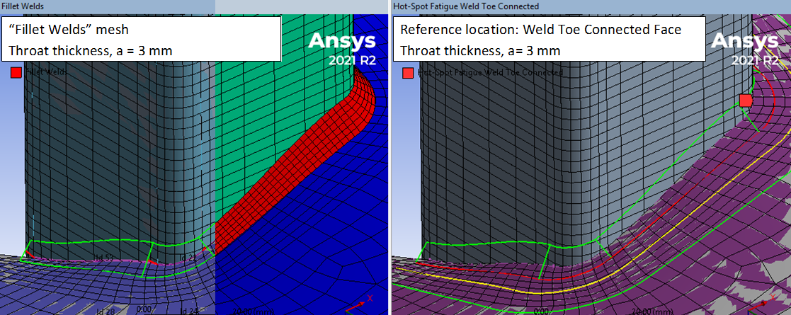
| Reference location | Reference Location from where to extrapolate stress. |
| Throat thickness | Weld throat thickness, a. Visible for Reference location “Weld Toe *” |
| Hot Spot Method | |
| Stress Type | Stress Types |
| Alpha (DNV) | Factor α (Used only for Stress Type “Equivalent (DNV)”) (i) |
| Extrapolation | Constant/Linear (Default)/Quadratic. Extrapolation method |
| Material thickness | Thickness, t, used to calculate the hot-spot extrapolation points, X (ii). |
| a | First extrapolation point coefficient. Xa = a·t. Default a = 0.4 (Yellow line). |
| b | Second extrapolation point coefficient. Xb = b·t. Default b = 1.0 (If “Quadratic” b = 0.9, Green line). |
| c | Third extrapolation point coefficient. Xc = c·t. Default c = 1.4 (Used only for “Quadratic”, Blue line). |
| Offset | Hot-spot edge offset on reference face normal to edge tangent (iii). |
(i) Alpha (DNV)
If FAT Class “DNV T.2-* C2”: α = 0.90, “DNV T.2-* C1”: α = 0.80, “DNV T.2-* C”: α = 0.72 DNV
(ii) Material thickness
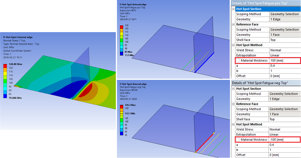
For shell models the thickness is extracted from the reference face. Default t = 0.0 mm. Must not be zero! Use a negative thickness to flip extrapolation direction in case the face continues on both sides of the edge, i.e. an “internal edge”.
(iii) Offset
Default = 0.0 mm. If Reference location = “Add weld *” the offset is defined by the throat thickness, see section Extrapolation graphics.
Reference Face
The hot-spot stress is calculated from node results on this face.
Only one unique face for each Hot-Spot edge is allowed.
If only one Hot-Spot Section edge is selected all reference faces are used for stress calculation.
Additional “unconnected” faces can be selected and used for the Reference Location = “* Unconnected Face”.
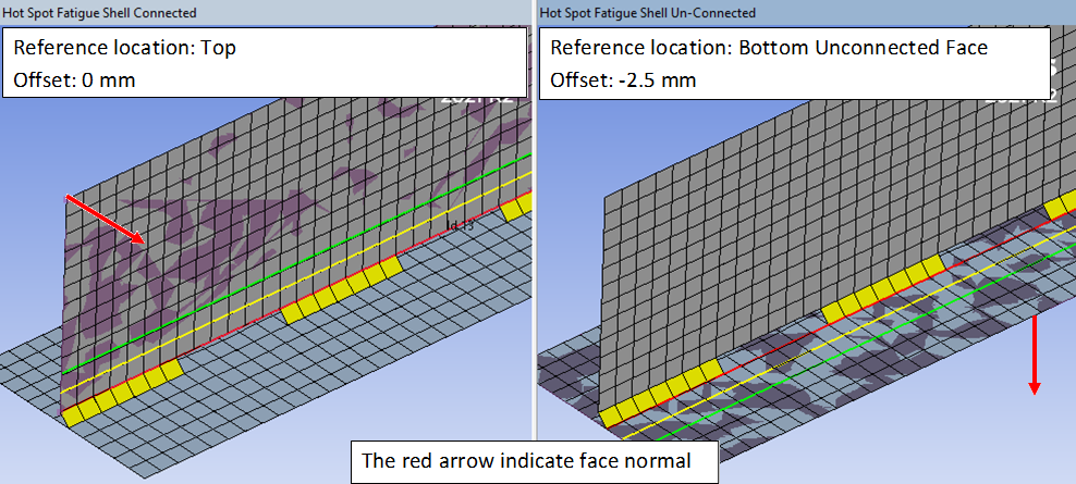
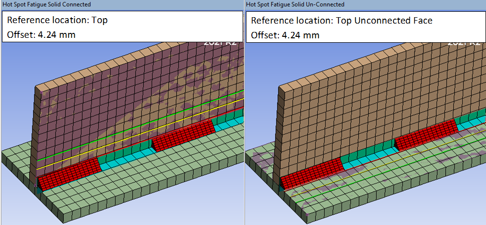
Reference Location
This property sets the location from where to extrapolate stresses. For a shell model “Top/Middle/Bottom” indicate the shell face side. This selection has no impact on a solid model.
The “* Unconnected Face” allows to post process on a “target” face not connected to the Hot Spot Section.
The “Weld Toe *” allows to post process “Add fillet weld” and will display the property “Throat thickness” to calculate the edge offset. This option will also display a wire frame graphics of the weld size in the same way as for the “Add fillet weld” feature. See section “Extrapolation graphics” for examples.
| Reference Location | Extrapolation from |
|---|---|
| Top | Shell face “Top” |
| Middle | Shell face “Middle” |
| Bottom | Shell face “Bottom” |
| Top Unconnected Face | (Shell face “Top”) of an unconnected face |
| Bottom Unconnected Face | (Shell face “Bottom”) of an unconnected face |
| Weld Toe Connected Face | Fillet weld reference face |
| Weld Toe Unconnected Face | Fillet weld target (unconnected) face |
The new “Weld” mesh feature from 2021 R1 allows to connect shell models with weld elements.
To post process on the “target face” include the face in the “Reference Face” scoping.
The direction of the hot-spot extrapolation lines and offset can be swapped by using a negative Thickness and negative Offset, see section Extrapolation Direction.
The “Unconnected Face” can also be used on solid models connected with contacts or “Add Fillet Welds”.
When welds are created using Add Fillet Welds the “Weld Toe * Face” option will calculate the local edge offset based on the Throat thickness, a. The weld geometry is plotted with a green wire frame.
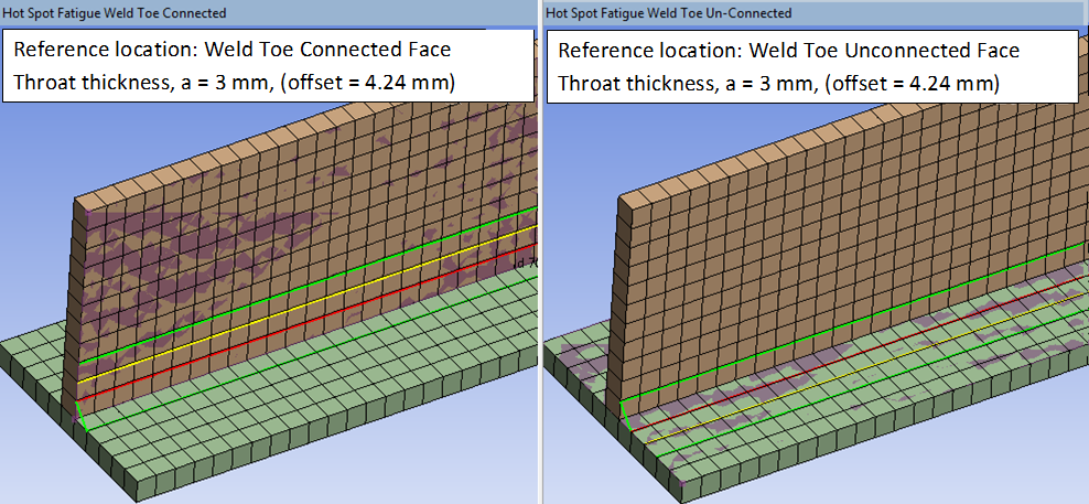
For welds with variable angle, α, the offset is calculated for each node, offset = a/cos(α).
Hot-Spot Method - Stress Type
| Stress Type | Description |
|---|---|
| Normal (Default) | Stress normal to the Hot-Spot edge, σn. |
| Parallel | Stress parallel to the Hot-Spot edge, σp. |
| Shear | Shear stress on the Hot-Spot reference face, τnp. |
| Shear (Max) | Maximum shear stress, τmax = sqrt((0.5·(σn - σp))2 + τnp2) |
| Principal (no limit) | Maximum principal stress, σprin = max(abs(σ1), abs(σ3)). |
| Principal (IIW limit) | Maximum principal stress (IIW), σprin (IIW) = σprin or σn (i). |
| Principal (Normal) | Principal stress within 45 deg from the Hot-Spot edge normal direction, σprin,n |
| Principal (Parallel) | Principal stress within 45 deg from the Hot-Spot edge parallel direction, σprin,p |
| Equivalent | Equivalent von-Mises stress, σeqv = sqrt(σn2 + σp2 - σn·σp + 3·τnp2) |
| Equivalent (DNV) | σeqv (DNV) = max(sqrt(σn2 + 0.81·τnp2), α·σprin) (ii) |
(i) Stress Type “Principal (IIW limit)”
If the angle, α, between the principal stress and extrapolation normal is greater than 60 degrees, the normal stress is automatically used, see IIW.
(ii) Stress Type “Equivalent (DNV)”
The “Equivalent (DNV)” is the implementation of the “DNV-RP-C203 effective hot-spot stress (eq. 4.3.1)”.
Extrapolation Graphics
Before the result is evaluated the extrapolation lines are shown to verify that they fall within the reference face and that the mesh is well defined. At least one unique node for each extrapolation line is needed. The extrapolation lines may be projected to the surface using the “Hot-Spot - Project lines on geometry” property in Weld Fatigue Settings. This setting will not influence the result quality.
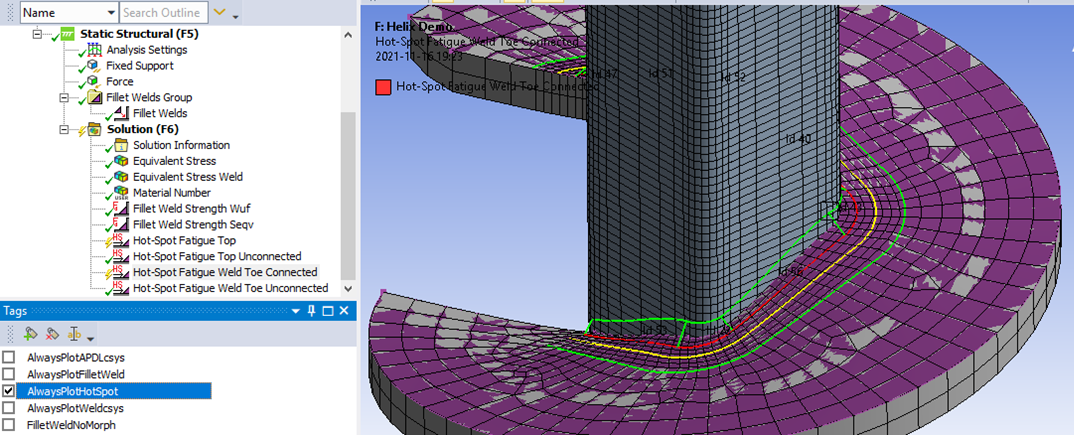
To always show the Hot-Spot extrapolation lines use the tag “AlwaysPlotHotSpot” on the result. The default setting can be changed using the “Hot-Spot - Always plot lines” property in Weld Fatigue Settings.

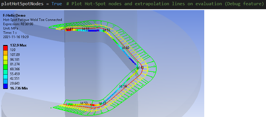
There is a debug option “Hot-Spot - Plot nodes (debug)” in the Weld Fatigue Settings that will plot the hot-spot nodes and extrapolation lines when evaluating a weld result. The line indicates the extrapolation normal and stress direction. If the geometry is curved the direction is projected onto the surface. When changing between evaluated results the nodes and lines will not be visible anymore.
If the lines that show the extrapolation locations are not displayed at the expected location the surface geometry quality may be poor. See the Debugging tips in the “Add Welds” section.
Extrapolation Direction
For models with T-junctions or internal edges the extrapolation direction can be switched by using a negative thickness. If the reference face is un-meshed the extrapolation lines may be shown at random side of the Hot-Spot edge.
Mesh requirements
The mesh must be fine enough to allow one or two elements between the hot-spot and the first extrapolation point as well as between the two (or three) extrapolation points.
The app will use a polynomial interpolation to calculate the stress at the extrapolation points, hence the mesh does not need to be a perfect mapped mesh with nodes at the extrapolation lines.
If the mesh quality is not good enough no fatigue result is displayed.
Weld Mesh method
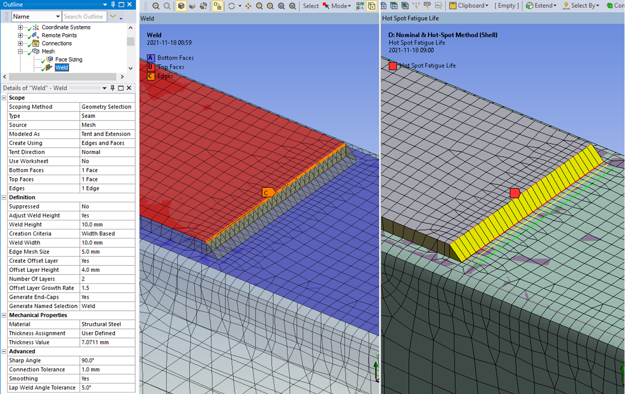
The weld mesh method (Ansys 2021 R1) can be used to generate a weld connection and create an imprint suitable for hot-spot method. See the demo model “Nominal & Hot-Spot Method (Shell)” in “WeldToolkit-FatigueDemos_V2XY.Z.wbpz”. For more info see the Ansys documentation Meshing User’s Guide>Local Mesh Controls>Weld.
Extrapolation comparison
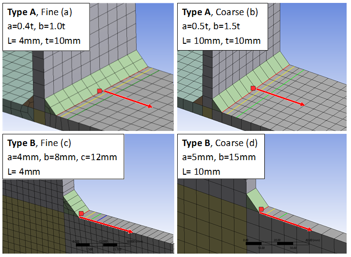
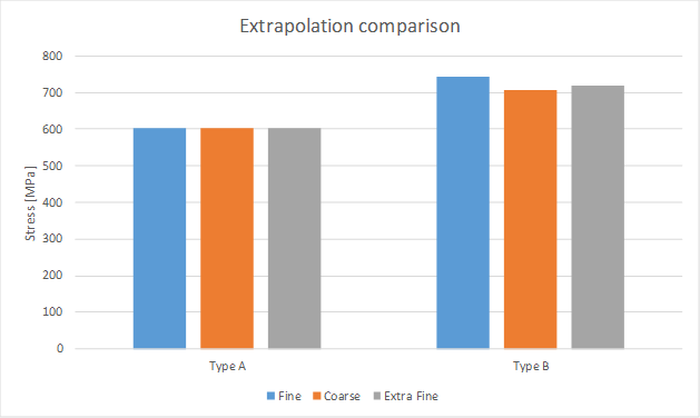
In IIW recommendations are made for mesh size, L, and extrapolation options for Type A and Type B geometry. In addition to the model mesh size 10 mm and 4 mm a model with mesh size 2 mm, “Extra Fine”, is included in the comparison.
For Type A the three models give the exact same Hot-Spot stress.
For Type B the coarse model gives slightly lower stress (un-conservative).
Hot-Spot Life Quality
The result item “Life quality” is an empirical factor of the ratio between the calculated life and the “true life”.
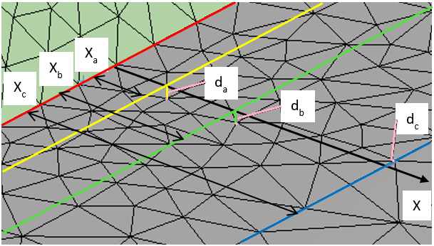
The Life quality is based on the distance, d, between the closest node to each extrapolation point. Optimal quality is 1.0. If the same node is found for all extrapolation points the quality is set to 0.0. Life quality = 1 - (da/Xa)2 - (db/(Xb-Xa))2 - (dc/(Xc-Xb))2 (Linear extrapolation uses a and b only)
The singularity at the “Hot-Spot” influences the stress at the first extrapolation point. A coarse mesh will usually result in a higher Hot-Spot stress and lower predicted life whereas a fine mesh allows the singularity stress to be eliminated before the first extrapolation point resulting in higher predicted life.
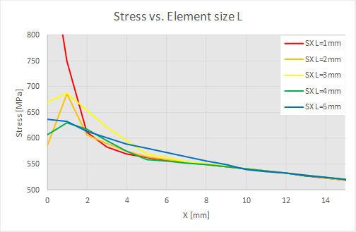
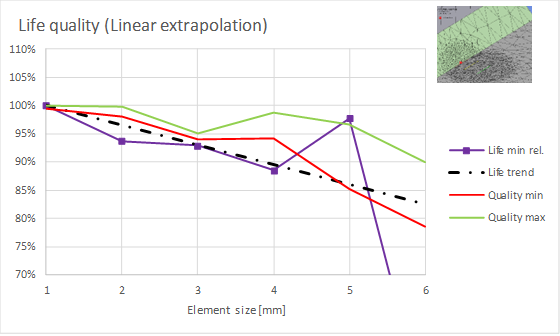
A parameter study of the element size, life and quality for a short segment of a tetrahedron mesh shows the following two graphs for linear and quadratic extrapolation.
Thickness, t = 10 mm, a = 0.4, b = 1.0
Thickness, t = 10 mm, a = 0.4, b = 0.9, c = 1.4
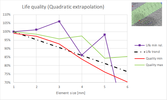
For increasing element size the variation of life and quality increases but the trend is that the result Life quality follows the calculated life.
For thickness 10 mm the recommended element size is 2 mm in order to have two elements before the first extrapolation point.
 Effective Notch Stress Fatigue
About
The effective notch fatigue method is usually used in a sub-model where the actual weld geometry is defined together with the notch radii. The notch result calculates the selected stress type in the notch fillet and plot the result on the connected edges.
Usage
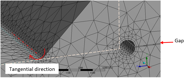
At the weld toe the notch radius can be added by a fillet feature. At the weld root the notch radius can be added by a Boolean cut operation. Make sure to include a gap between the plate parts and place the notch cut so it does not reduce the effective throat thickness, see dashed lines in the figure below.
Fillet radius R = 1 mm is valid for thickness ≥ 5 mm IIW. For thinner parts R = 0.05 mm may be used but other recommendations exist such as R = 0.3 mm. The app will not check the notch radius or part thickness.
The FAT class depends on material, notch radius and stress type. Common values are found in the table below IIW.
| Material | R = 1 mm | R = 0.05 mm |
|---|---|---|
| Steel | FAT 225 | FAT 630 |
| Aluminum alloys | FAT 71 | FAT 180 |
| Magnesium | FAT 28 | FAT 71 |

| Effective Notch Edge | |
|---|---|
| Scoping Method | Geometry Selection/Named Selection |
| Geometry | Edges of solid bodies along the notch fillet used for plotting the result. (Red line) |
| Effective Notch Face | |
| Scoping Method | Geometry Selection/Named Selection |
| Geometry | Non-planar notch faces of solid bodies connected to the notch edges. (Purple faces) |
| Effective Notch Method | |
| Stress Type | Stress Type |
| Exclude boundary nodes | Yes (Default)/No Do not display fatigue results for nodes on boundary conditions. |
Effective Notch Method - Stress Type
| Stress Type | Description |
|---|---|
| Tangential (IIW default) | Stress normal to the Notch edge (tangential), σn |
| Parallel | Stress parallel to the Notch edge (axial), σp. |
| Principal | σprin = max(abs(σ1), abs(σ3)) |
| Sum of Principal | σsum = σ1 + σ2 + σ3 |
| Stress Intensity | σint = max(abs(σ1 - σ2), abs(σ2 - σ3), abs(σ3 - σ1)) |
| Equivalent | σeqv = sqrt(0.5·(σX - σY)2 + (σY - σZ)2 + (σZ - σX)2 + 6·(σXY2 + σYZ2 + σXZ2)) |
| Shear (Max) | τmax |
Equivalent is the signed von-Mises Equivalent stress. Sign taken from the largest principal stress.
Notch Mesh, Graphics and Result evaluation
The notch mesh must be fine enough to allow at least four second order elements for a 90-degree segment, i.e. element length 0.4 mm in a R = 1 mm notch radius. Use inflation layers or sphere/body of influence to get good element quality.
When opening a project saved with previous app version it is required to assign an edge scoping before you may evaluate.
The result in the notch fillet is displayed on the nearest notch edge node.
Nodes from elements connected to a cut boundary section or other displacement constraints are automatically excluded from the evaluation by setting the property “Exclude boundary nodes = Yes”. This sets the “Life quality” to zero and will avoid the stress singularity at the boundary condition to influence the fatigue result, see example below.
There is a debug option “Effective Notch - Plot Notch Vectors” in the Weld Fatigue Settings that will plot the notch stress direction vectors when evaluating the weld result. When changing between evaluated results the vectors will not be visible anymore.
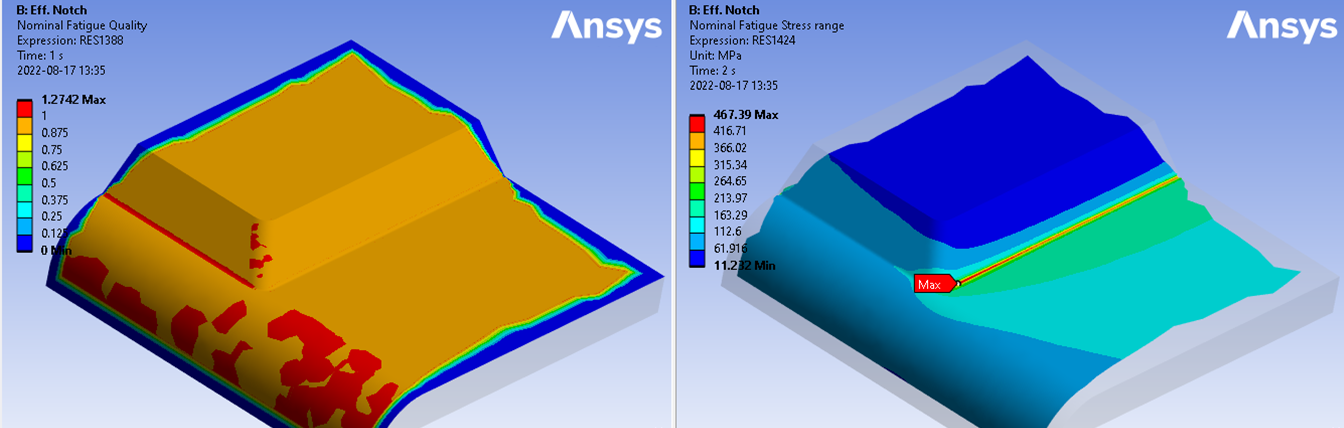
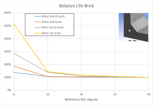
Notch Life Quality
The expected life is highly sensitive to the stress range. A stress convergence study shows that 2nd order brick elements require 24 elements/360 degree, and first order elements require 40 elements/360 degree.
The result “Life quality” is the ratio between the calculated life and the “true” life as a function of normal angle difference, phi, over the element. A coarse mesh over predicts the life so dividing the calculated life with the quality is a rough estimate of the “true” life.
Second order tetrahedron elements tend to give higher stress compared to brick elements for the same mesh resolution and are therefore conservative. First order tetrahedron elements must never be used. Using inflation layers on a tetrahedron mesh improves the result and is recommended practice.
The Nominal method uses the same definition for “Life quality” for solid models.

Output
The Weld Fatigue object writes a property and result csv files to the solver files directory of the analysis. These files are used by the Worksheet Preview and Weld Report features and can easily be imported to Word or Excel.
Output csv files
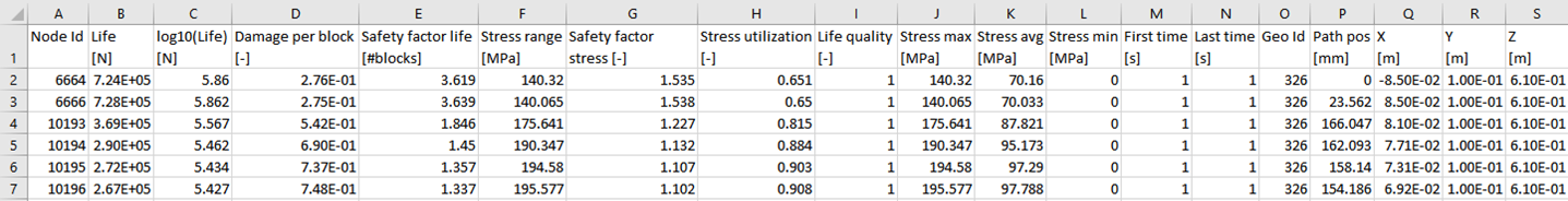
In addition to the available Result Items the csv file contains node, geo and coordinate information. The table is sorted in “Path pos” for each group of edges to do graphs in e.g. Excel. The data can also be sorted using the X, Y, Z coordinates if needed.
| Result Item | Description |
|---|---|
| Node Id | Node numbers from result object. |
| Geo Id | Face or edge Id number. |
| Path pos | Edge path position. |
| … | … |
| X | Node X coordinate in global system. |
| Y | Node Y coordinate in global system. |
| Z | Node Z coordinate in global system. |
The csv file name will not change if the result is renamed. Clear and evaluate to re create the csv file.
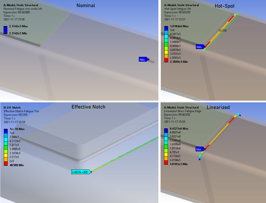
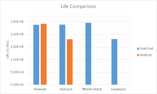
Comparison of fatigue methods
The four fatigue methods show similar results where Nominal and Hot-Spot method has identical life, Effective Notch method has 1% higher life and Linearized has 24% lower life compared to the Nominal method respectively.
For a shell model (1st order) the Hot-Spot method life is 25% lower compared to Nominal.
In this test the new “Weld” mesh method is used to create the weld mesh including the mesh imprint for Hot-Spot extrapolation, see the section Weld Mesh method in the Hot-Spot section.
The Hot-Spot result is very sensitive to the mesh method, size and quality at the hot spot, e.g. solid vs. shell, contact vs. multi-body, with or without weld elements. In this example the Hot-Spot life could differ as much as 50% compared to the Nominal life.
Verification
A number of fatigue verification models can be downloaded from the “Demo and verification models” found in the Downloads section. A verification report can be automatically created by using the Weld Report feature. Individual results can be studied using the Worksheet Preview feature.
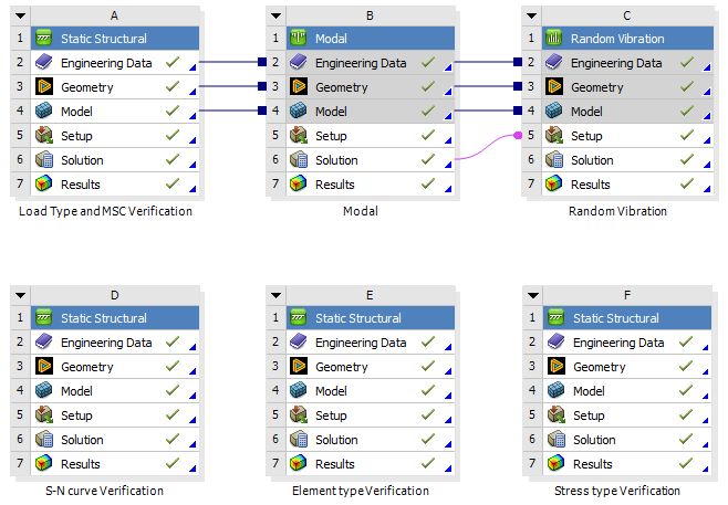
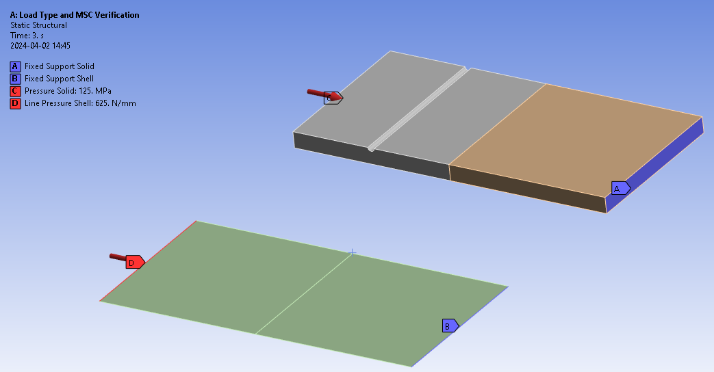
A: Load Type and MSC Verification
The model is intentional oriented at a random angle with respect to the global coordinate system. The load case LC1 is uniaxial so that the stress SX = S1 = Seqv = 125 MPa. LC2 = 0.1*LC1 and LC3 = -LC1.
Tests performed are:
- Scoping options: [Geometry Selection, Named Selection, Nodal selection]
- Stress type: [Normal, Principal, Equivalent etc.]
- Load case: [Zero Based, Fully Reversed, Ratio, Load Combination, Load Scanning, Solution Combination, Solution Scanning, Random]
- Load scale factor
- Mean Stress Correction Theory: [None, Goodman, Soderberg, Gerber, ASME Elliptical, Modified Goodman]
- Linearized Parent and Child result.
- Cumulative Damage and Fatigue Child result.
B: Modal
Used as input for Random Vibration analysis.
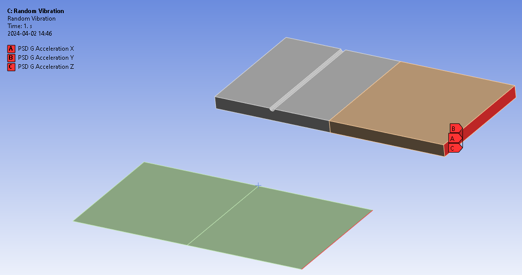
C: Random Vibration
The load case is a uniform “PSD G” spectrum applied in all three directions.
Tests performed are:
- Weld Strength [Butt Weld Strength, Butt Weld Strength Shell]
- Weld Fatigue [CSV, Linearized, Nominal, Hot-Spot, Effective Notch]
- Statistical Average Frequency, SAF
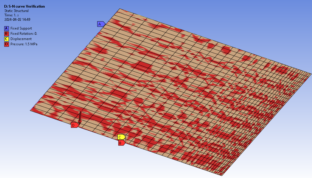
D: S-N curve Verification
The shell model is fixed in one end and loaded with a pressure to generate a variable stress along the surface. The mesh is biased to create more nodes towards the free end so the stress points are distributed better in a log-log S-N graph.
The Nominal Fatigue life is calculated for each available FAT class S-N curve along the edges and are compared with original S-N graph.
The FAT class S-N curves for IIW, Eurocode 3, Eurocode 9 and DNV are verified in the corresponding folder in the “Solution”.
The stress range and calculated life (from the csv files in the working directory) is plotted on top of the original S-N curve in Excel, see the file “Verification FAT.xlsx” and “Verification FAT EC9.xlsx” in the project “user_files”. The graph for a sample of curves is shown in each folder.
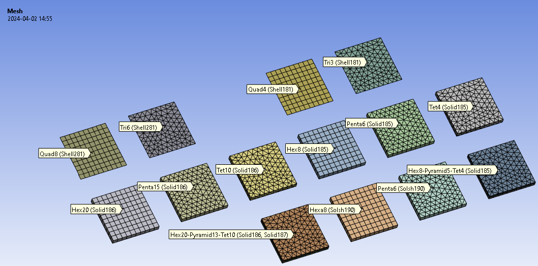
E: Element type Verification
A bending load case is defined to study the stress at “Top” and “Bottom” for all mesh and geometry types.
The “Weld Settings” option “Signed stress range = Yes” is used together with “Result Item = Stress Range” (instead of “Stress Max” or “Stress Min”) to compare the stress with the native “Normal Stress” result with correct sign.
Tests performed are:
- Geometry [Shell, Solid, Solid-Shell]
- Element order [Linear, Quadratic]
- Element types [Tri, Quad, Tet, Pyramid, Penta, Hexa]
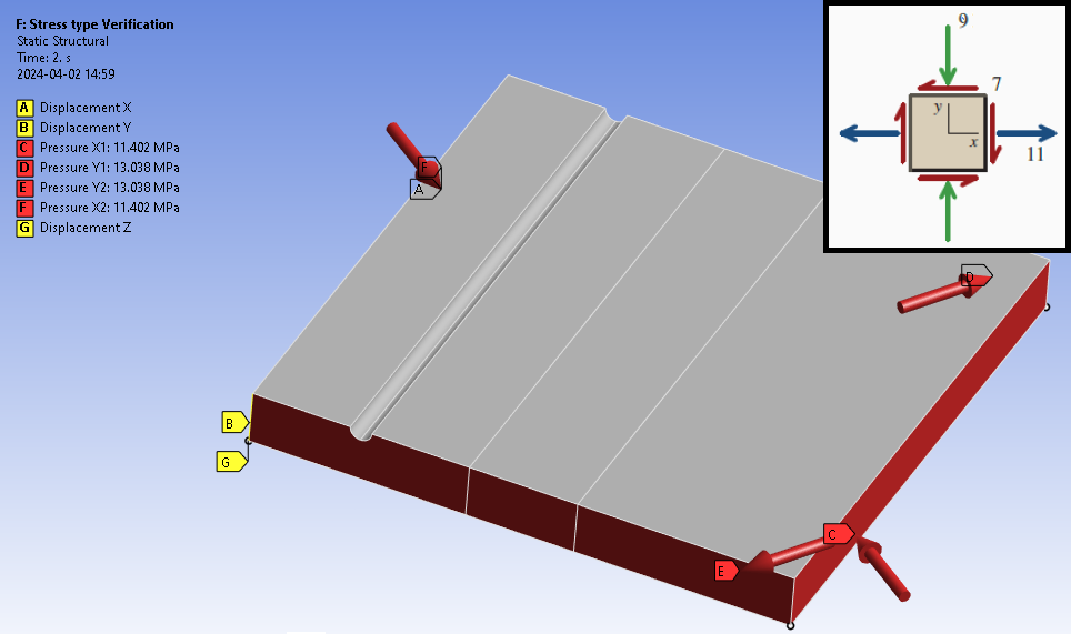
F: Stress type Verification
A bi-axial stress state is defined that changes direction between the load steps creating a non-proportional load case (S_XX = 11 MPa, S_YY = -9 MPa, S-XY = 7 MPa).
The resulting principal stresses are; S1 = 13.21 MPa, S2 = -11.21 MPa
The angle of principal stress relative to X; phi_1 = -17.5 deg, phi_2 = 72.5 deg
The resulting maximum shear stress; T_max = 12.21 MPa
The weld fatigue stresses are compared with native stresses and “User defined” stresses.
Tests performed are:
- Nominal: [Normal X, Normal Y, Shear XY, Principal, Sum of Principal, Stress Intensity, Equivalent, Shear (Max)]
- Hot-Spot: [Normal, Parallel, Shear, Shear (Max), Principal (no limit/IIW limit/Normal/Parallel), Equivalent, Equivalent (DNV)]
- Effective Notch: [Tangential, Parallel, Principal, Sum of Principal, Stress Intensity, Equivalent, Shear (Max)]
- Load cases: [Zero Based, Load Combination, Load Scanning]
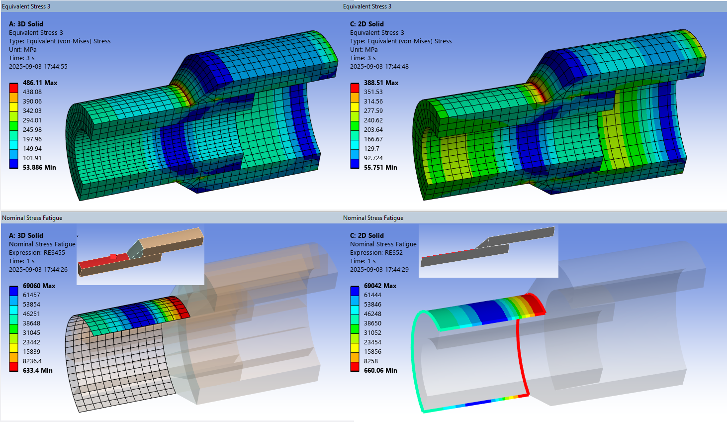
Axi-symmetric models
Weld Fatigue can be used with “Symmetry” boundary conditions (“Symmetric” and “Axi-symmetric”) both in 3D (solid, shell) and 2D (solid). A new verification model Axisymm_fatigue_2025R2.wbpz demonstrates the capabilities and what fatigue methods that can be used with each model.
3D Solid sector (left) vs. 2D Solid sector (right)
Add Welds cannot be used since the Symmetry boundary is not applied on the ends of the weld. Use a Virtual Weld with a “Manual select weld part” instead.
Select the edges of a 2D solid to post process the outer faces using CSV Stress Fatigue or Nominal Stress Fatigue. Hot-Spot Stress Fatigue may be used to extrapolate stresses through the thickness in a similar way as Lineraized Stress Fatigue.
In previous versions (< 2025R2) you needed to set “Shell Position = Bottom” in the 2D analysis to get correct values for the “shell” elements.
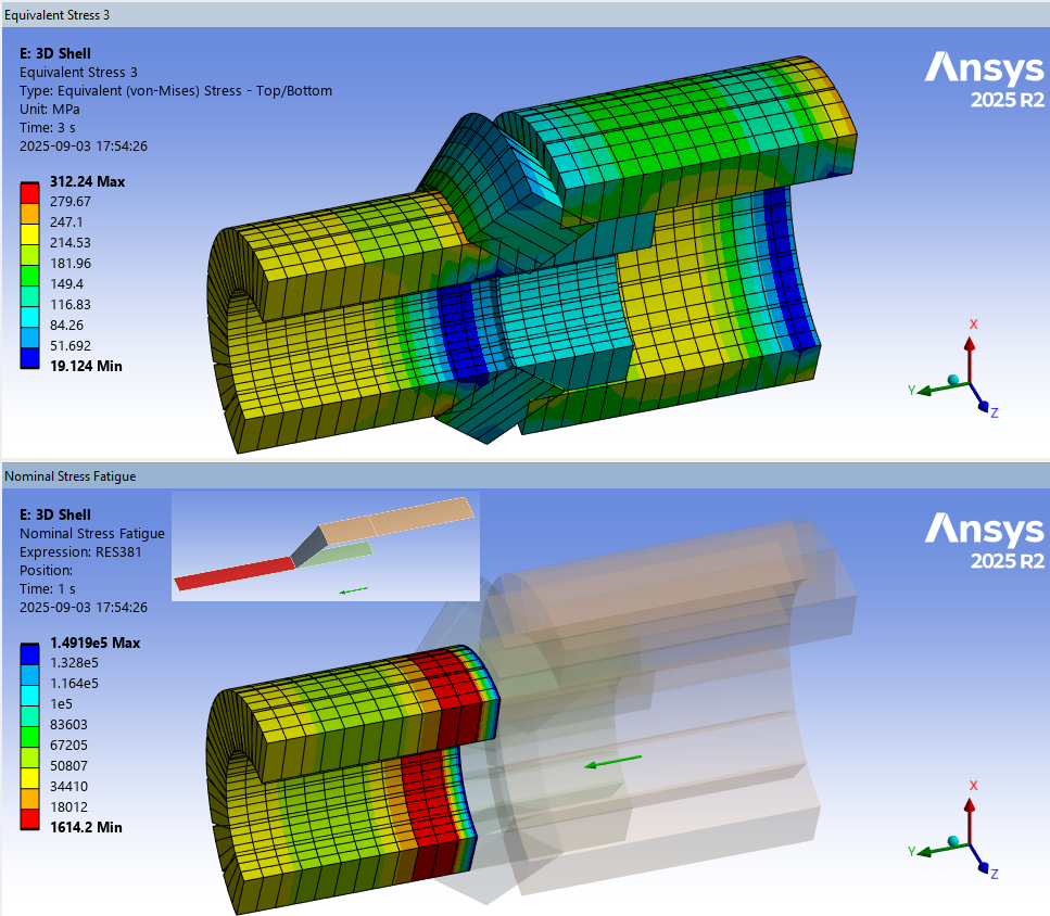
3D Shell sector
Use “Shell Position” as normal, in this case “Shell Position = Top” to evaluate on the shell top side.
Validity of the fatigue results
In stress-life fatigue calculation the stress range should be within the limits of the elastic properties of the material. The method should not be used for:
- Low cycle fatigue (strain based fatigue).
- Corrosive conditions.
- Elevated temperature operation in the creep range.
It is the user’s responsibility to ensure that the FE-model, chosen fatigue method, input values and results obtained by this application is suitable for his/her intended purpose, e.g. to evaluate according to a specific design code or to apply fatigue modification factors due to misalignment etc.
Also see the new standard: EN 1993-1-14:2025 Eurocode 3: “Design of steel structures - Part 1-14: Design assisted by finite element analysis”.
Stress range check
The IIW recommendations for stress range check are implemented for Nominal and Hot-Spot Method based on the Yield Limit (Ry) defined in the Mean Stress Theory property.
If the following conditions are not fulfilled a warning message is issued.
- Nominal stress range Δσnom < 1.5·Ry or max stress Δσnom < Ry
- Hot spot stress range ΔσHS < 2·Ry or max stress σHS < Ry
Use the results “Stress range” and “Stress max/min” to review the condition. Also verify the fatigue resistance of the parent material.
All IIW and DNV GL S-N curves are limited by the parent material (FAT160 & B1)